My first encounter with four-dimensional polytopes was Jenn 3D (2001-2007) by Fritz Obermeyer. Jenn describes itself as follows:
Jenn is a toy for playing with various quotients of Cayley graphs of finite Coxeter groups on four generators. Jenn builds the graphs using the Todd-Coxeter algorithm, embeds them into the 3-sphere, and stereographically projects them onto Euclidean 3-space.
Wow. This description made absolutely no sense to me when I first read it - none of these terms were familiar to me. My purpose with this page is to go through this description step-by-step and explain the various terms.
We will also go one step further, and discuss how these structures can be ray traced in realtime. This can be done using a clever (inverse) construction technique of folding space into a fundamental domain. The technique was originally described by Abdelaziz Nait Merzouk (aka Knighty) in a Fractal Forums thread from 2012.

Symmetries of the cube
We will start out in three dimensions with a familiar object: the cube.
The cube has several automorphisms - transformations that will map the cube onto itself. For instance, we can easily find several rotations (between opposite vertices: 4 (120 degrees), opposite mid-edges: 6 (180 degrees), and opposite faces: 3 (90 degrees): a total of 4*2+6*1+3*3 = 23 rotations.
Including the identity transformation, and taking into account that we could also mirror each one of these transformations, we arrive at 48 automorphisms for the cube.
Besides the rotation symmetries above, we can also depict the reflection symmetries. Shown to the right are the 9 different such reflection operations, that will map the cube onto itself (although in a mirrored version).
These 48 transformations form a group: a set of elements, together with a rule for combining any two elements such that the result is again an element in the set. There must an identity element in the group, and every element must have an inverse element: i.e. an element such that combining the element and its inverse results in the identity element.
In our case, combining any number of the 48 transformations will result in a transformation that is already present in our set of transformations. Likewise, for all rotations and reflections, there exists an inverse transformation (for 180 degrees rotations, and for reflections, the transformations are their own inverses).
These transformations are not independent: some transformations can be expressed by combining other transformations. Perhaps it is possible to find a smaller subset of transformation that could be combined to form all the 48 automorphisms?
This is known as a set of generators: a subset, S, of elements in the group G, which can be used to express all elements.
For the cube, it is possible to find a set of three reflections, which can be used to form all the 48 transformations. One such set is shown to the right: here we have three reflection planes, which we could think of as operators - let us call them R, G, and B after their colors. This set can be used to construct all other transformations.
Notice that the angle between the reflection planes (sometimes called mirrors) is: $$\angle(R,G) = 45^{\circ} $$ $$\angle(G,B) = 60^{\circ} $$ $$\angle(R,B) = 90^{\circ} $$
Now, combining two reflections results in a rotation of twice the angle between the reflection planes. So applying e.g. GB would be equal to a rotation of 120 degrees. And applying GB three times, e.g. GBGBGB, would not change the input.
This means we can establish the following relations between the generators:
$$R^2 = B^2 = G^2 = (RG)^4 = (GB)^3 = (RB)^2 = I$$Given a set of generators, how many different elements are there in our set? And can we decide whether two compositions (say RGRG and RBG) are identical operations? This turns out to be a computationally hard problem, known as the word problem for groups. But for some specific groups, this problem is computationally tractable.

The Todd-Coxeter Algorithm
Our example relations above form a special group, called a Coxeter group. That is a group where the generators have relations of the form: \((ab)^{m_{ab}}\), as above: $$(RG)^4 = (GB)^3 = (RB)^2$$ The generators must also be their own inverse: $$R^2 = B^2 = G^2$$ Since the generators are their own inverses, they can be associated with reflections.
For Coxeter groups, it is possible to identify all elements in the group, given the generators. The Todd-Coxeter Algorithm provides a way to identify and count all elements generated by our generators. (Quick digression: The Todd-Coxeter algorithm was one of the first non-numerical algorithm to be implemented on a digital computer - using an EDSAC 1 in 1953)
Actually, the Todd-Coxeter algorithm does a bit more than counting the elements: it also allows for enumerating all cosets of G, for a given subgroup H.
What does this mean?
A coset is the set resulting from multiplying all members in \(H\) by a group element \(g\) from \(G\). A (left) coset is written \(gH\). The number of cosets is written \(|G:H|\). Lagrange's theorem states that \( [G:H]={|G| \over |H|} \). All the cosets for a given subgroup form a new set, called a quotient set (denoted G/H).
The algorithm works by keeping track of several tables: a coset table (listing the generator actions on the different cosets), a subgroup table (listing subgroup generator actions), and a table for each relation between the group generators. The algorithm works by filling out rows in these tables. Once a row is closed, a (potentially) new piece of information is known.
Here is a demo (use the 'step' button to fill the table):
Group: Subgroup: Step
Let us look at the various cosets you get when you use Todd-Coxeter on the symmetry groups for the regular polytopes, using different subsets of the generators to specify a subgroup:
| Subgroup cosets | ||||||
|---|---|---|---|---|---|---|
| Name | Diagram | Generator relations | Automorphisms | g,b | r,b | r,g |
| Tetrahedron | COX(3,3) | \((rg)^3\),\((gb)^3\);\((rb)^2\) | 24 | 4 | 6 | 4 |
| Cube | COX(4,3) | \((rg)^4\),\((gb)^3\),\((rb)^2\) | 48 | 8 | 12 | 6 |
| Octahedron | COX(3,4) | \((rg)^3\),\((gb)^4\),\((rb)^2\) | 48 | 6 | 12 | 8 |
| Dodecahedron | COX(5,3) | \((rg)^5\),\((gb)^3\),\((rb)^2\) | 120 | 20 | 30 | 12 |
| Icosahedron | COX(3,5) | \((rg)^3\),\((gb)^5\),\((rb)^2\) | 120 | 12 | 30 | 20 |
| Vertices | Edges | Faces | ||||
| Subgroup cosets | |||||||
|---|---|---|---|---|---|---|---|
| Name | Diagrams | Generator relations | Automorphisms | g,b,a | r,b,a | r,g,a | r,g,b |
| 5-cell | COX(3,3,3) | \((rg)^3\),\((gb)^3\),\((ba)^3\),\((rb)^2\),\((ra)^2\),\((ga)^2\) | 120 | 5 | 10 | 10 | 5 |
| 8-cell | COX(4,3,3) | \((rg)^4\),\((gb)^3\),\((ba)^3\),\((rb)^2\),\((ra)^2\),\((ga)^2\) | 384 | 16 | 32 | 24 | 8 |
| 16-cell | COX(3,3,4) | \((rg)^3\),\((gb)^3\),\((ba)^4\),\((rb)^2\),\((ra)^2\),\((ga)^2\) | 384 | 8 | 24 | 32 | 16 |
| 24-cell | COX(3,4,3) | \((rg)^3\),\((gb)^4\),\((ba)^3\),\((rb)^2\),\((ra)^2\),\((ga)^2\) | 1152 | 24 | 96 | 96 | 24 |
| 120-cell | COX(5,3,3) | \((rg)^5\),\((gb)^3\),\((ba)^3\),\((rb)^2\),\((ra)^2\),\((ga)^2\) | 14400 | 600 | 1200 | 720 | 120 |
| 600-cell | COX(3,3,5) | \((rg)^3\),\((gb)^3\),\((ba)^5\),\((rb)^2\),\((ra)^2\),\((ga)^2\) | 14400 | 120 | 720 | 1200 | 600 |
| Vertices | Edges | Faces | Cells | ||||
An interesting structure emerges here: looking at the cosets for the subgroups generated by leaving out one of the generators, the number of cosets matches the number of vertices, edges, or faces! It seems we can fully describe the geometric structure by forming various quotient sets.
Also notice, that the ordering matter here: the cube and octahedron have the same generators (just switch 'r' and 'b'), and same symmetry group, but the number of faces and vertices are swapped. These shapes are said to be dual. The Dodecahedron/Icosahedron, the 8-cell/16-cell, and 120-cell/600-cell all form dual pairs.
So what differentiates a cube from an octahedron? The answer is, that it depends on how the initial vertex is placed. Notice the outer circle on the first reflector, r, in the Coxeter diagram: this circle specifies that the initial vertex should be placed somewhere off the reflection plane for r, but on the reflection planes for g and b. (This also means that the initial vertex would be taken to itself when applying g and b).
Let us explore the quotient sets a bit more: how do we generate the geometry and how do we associate edges with vertices?

Generating geometry from group structure
We will recreate the Euclidean geometry from the abstract Coxeter group description.
Given the generator relations, we know the angles between the reflector planes: If there is a relation on the form: \((RB)^{N}\), the angle between the reflection planes R and B must be \( \pi / N \) - which again corresponds to a rotation of \( 2\pi / N \) degrees. For the cube the angles between the reflection planes are 45, 60, and 90. The first step is to create a set of reflection plane normal vectors with these angles between them. This can be done iteratively, by starting with an arbitrary unit vector, and adding vectors at corresponding angles, e.g.:
$$ \begin{pmatrix} & 1 \\ & 0 \\ & 0 \end{pmatrix}, \begin{pmatrix} & cos(\theta_{12}) \\ & N_1 \\ & 0 \end{pmatrix}, \begin{pmatrix} & cos(\theta_{13}) \\ & \frac{cos(\theta_{23})-cos(\theta_{12})cos(\theta_{13}) }{N_1} \\ & N_2 \end{pmatrix} $$
These vectors are the normals of the reflecting planes (The N's are normalization constants that can be trivially calculated - all the normals must be unit length).
We now have our reflection planes (the group generators) defined. Given a starting point, we can apply these and create the full geometry. But how do we choose the starting point? As previously mentioned the cube and octahedron share the same generator relations (they are dual). So why are they different? Looking at their coxeter diagram in the table above, this has to do with the special outer circle. This outer circle has a special meaning: the initial starting point should be located on the two other reflection planes (the blue and the green), but not on the red one.
We can use Gram-Schmidt orthonormalization to create a vector that is contained in the blue and the green plane, but not in the red plane. We do this by starting out with the three reflection plane normal vectors in the order blue, green, and red. After applying Gram-Schmidt to this set of vectors, the last vector in the transformed set will be orthogonal to the blue and green reflection plane normal vectors (and thus be located on the intersection of these two planes). The advantage of using Gram-Schmidt is that we can generalize this to four dimensions - if we had used the cross product, that would not have been possible.
The example below shows how this works for the dodecahedron. Like the cube, the dedocahedron can be generated by three generators, with angles 36, 60, and 90 degrees between the reflecting planes.
The table can be used to explore how the different quotient sets ties the vertices, edges, and faces together. Try hovering an entry.
For instance, see how vertex V0 connects to three edges (E0,E1,E3) and three faces (F0,F1,F2). Likewise, edge E0 connects two vertices (V0,V1) and two faces (F0, F1). The face F0 connects five vertices (V0,V1,V2,V3,V5) and five edges (E0,E1,E2,E4,E6)
Also notice the volume enclosed by the three arrows. This is the fundamental domain, which will we return to in the next section.

Ray tracing reflection groups
I have long been a fan of ray marching, and distance estimation techniques.
The previous section showed how to construct geometry by explicitly calculating positions for vertices, edges, and faces, and then displaying the structures by rasterizing polygons (using WebGL).
But it is possible to construct very efficient distance estimators for the reflection group polytopes - including the four-dimensional ones. Utilizing modern GPUs, this makes it possible to ray trace high-quality images in real-time.
This technique was originally described by Knighty in this Fractal Forums thread from 2012.
The basic idea is a clever trick: instead of trying to calculate the positions of all vertices and edges, we will first transform (using the group reflections) all points in space into the same 'fundamental' region or domain. The basic building block will be a fold: a simple conditional reflection - if we are on the wrong side of a reflection plane, we will do the reflection - otherwise not. Once our paths of folds ends in the fundamental domain, we can quickly test whether we are inside a vertex, edge, or plane (at least after assigning a width to these objects). We can also calculate the distance to the nearest part of the structure this way.
Being able to calculate the distance to the nearest part of a structure is very powerful. Given this distance estimator, we can render our object using ray marching: we can take steps along a ray from the camera, and stop once we are sufficiently close to the object. The distance estimator tells us how large steps we are allowed to march. And, since we now know how to determine how an arbitrary ray intersects our structure, we can ray trace it, including shadows and reflections. I previously described the technique here for a recursive tetrahedron.
The illustration above shows how to fold a point in space (the red ball) back into the fundamental domain (move to this region). You can move the red ball using the controls. By repeatedly applying the folds, we can trace a piecewise linear path back to the fundamental domain (the white ball shows the end point in the fundamental domain). Once in the fundamental domain, we can calculate the distance to the initial vertex: this distance is shown by the thin white line. Due to the symmetries, this is the same as the distance to the closest vertex of the red ball! The distance is visualized as the radius of the red sphere centered on the red ball.
How many folds do we need? It seems like the worst case is when the point is located in "mirrored" fundamental domain (move to this region). In this domain, 15 folds (3 generators x the max symmetry of 5) are required.
It may not seem the advantage is that big: we could have explicitly calculated the 20 vertices and 30 edges and calculated the distances to those. But for more complex structures (the 120-cell has 600 vertices and 1200 edges), the advantage is huge: the number of regions that can be folded back into a fundamental domain grows exponentially with the number of fold operations. And fold operations are cheap: for instance, in the example above, two of the reflections are orthogonal and can be aligned with the coordinate system axes. In that case, the fold operation may be implemented simply by taking the absolute value of the coordinates, e.g. pos.xy = abs(pos.xy). A very fast operation!
The folding approach also has another advantage: we do not require the elaborate coset structure of the symmetry group to figure out how the vertices are organized into edges and faces. We only need to describe the fundamental domain, then symmetry will take care of the rest.
Now we are ready for a real example of ray tracing a system of three generators:
In the example above, the U, V, and W parameters control the position of the initial vertex as specified in a coordinate system where each axis lives on the intersection of two reflection planes (the same coordinate system as defined in the dodecahedron example with the red, green, and blue arrows).
When the 'displayFundamental' option is enabled, the initial vertex will be displayed by a black line. The U,V, and W vectors are shown as white lines, and define the fundamental region (and any pair of white lines span a reflection plane).
When only U is enabled (i.e. non-zero), we get a regular polyhedron. But when we enable some of the other mirrors, we will get various uniform polyhedra. For instance, only enabling W will give us the dual of the original regular polyhedron. Enabling U and V will give us a truncated polyhedron.
The Degree parameter controls one of the angles between the reflection planes (e.g. 3 = 60 degrees, 4 = 45 degrees, 5 = 36 degrees). The two other angles are always 90 degrees and 60 degrees.
Notice, that the resulting structures are all convex, but not necessarily regular polytopes.

The fourth dimension
To get to the fourth dimension, we need one additional trick: the stereographic projection.
Stereographic projection is a projection from the surface of a sphere (in 3D) to a plane in 2D. In the example above, we have our cube embedded in a sphere in 3D. Notice, that the vertices will all be on the sphere surface - this is true for all regular polyhedra, also in four dimensions.
The edges of the cube are black. These are projected (the red lines) by following a point on the top of sphere, through the vertex, and down on the plane. The projection edges are drawn in green.
It is possible to rotate the cube using the controls. Notice, how the edges are curved when projected down onto the plane, even though they are straight in the cube. That is a choice: this corresponds to 'inflating' the cube onto the sphere, making the edges live on the great circle arcs.
The stereographic projection can be generalized to higher dimensions. This is how we will create our depictions of four dimensional polytopes. We will start out with a 3-sphere in four-dimensional space. The vertices of the polytopes will be placed on the surface of the 3-sphere, and we will make a projection onto 3-dimensional space.

Putting it all together
Here is the final example - ray tracing a system of four generators:
Similar to the 3D example, the U, V, W, and T parameters control the position of the initial vertex and the Degree parameter controls one of the angles between the reflection planes.
There is a set of controls for rotating the 4D object - this is similar to rotating the cube before projecting it down onto the plane in the previous illustration. Notice, that the rotation is not a true 4D rotation - only three coordinates get rotated. For some rotational values, the image gets fuzzy - I think this is when a vertex is close to the projection point of the 3-sphere and gets blown up.
The presets can be used to quickly toggle between the regular 4D polychora.
There is one technicality that has to be taken into account when ray marching 4D polytopes. We march the ray in three dimensions - so in order to get the distance estimates we do an inverse stereographic projection to get to a four dimensional point (see also Knighty's original description).
Once in 4D, we can calculate the distance estimate by folding the point back into the fundamental domain.

In Summary
Many different geometric objects can be described by their Coxeter diagram, e.g. . This diagram describes the structure of the symmetry group by defining relations between the generators. The generators can be interpreted as reflections - and the power of the pair-wise relations describes the angle between the reflection planes.
The Todd-Coxeter algorithm makes it possible to construct all elements in the symmetry group only from the description of the generator relations. It also allows us to find all cosets for a given sub-group. As we saw, by looking at the cosets for generator subgroups, we can identify edges, faces, and cells.
Based on this we can construct an explicit geometry by choosing a starting point and applying the group transformations. For the regular polytopes, the initial vertex must be placed on the intersection of all reflection planes, except one.
Instead of explicitly constructing all vertices, edges, and faces, it is possible to use a different approach: we can construct a function that for each point in space determines how close we are to a vertex or an edge - a distance estimator. We can do this by folding a given point in space repeatedly, until we reach our fundamental domain. This is powerful, because there are efficient methods for ray marching distance estimators (and it parallellizes trivally on GPU's).
All of the above will work in any number of dimensions. However, in order to do the actual visualization, we used (inverse) stereographical projection to reduce the number of dimensions from four to three.
Group theory and symmetries have been studied extensively by the math community, but most of the results are not very accessible unless you are a trained mathematician.
This page is barely scratching the surface. I hope to get some time to look into hyperbolic geometries and honeycombs, both of which would fit naturally together with the regular polytopes - but until then take a look at some of the links below.
A secondary goal with this project was to build a more engaging and interactive web presentation than the static blog entries I usually write - I have been very impressed with what has been happening on sites like Bret Victor's Worry Dream and Distill.pub. My most important lesson learned here, is that building interactive presentations do take up a lot of time (duh). Some of this was partly because I needed to learn new techniques and create a couple of tools from scratch (like building a small three.js framework for ray tracing - including automatic generation of an UI for setting the uniforms). I plan to carve out some of these tools to make them easier to reuse for future projects.
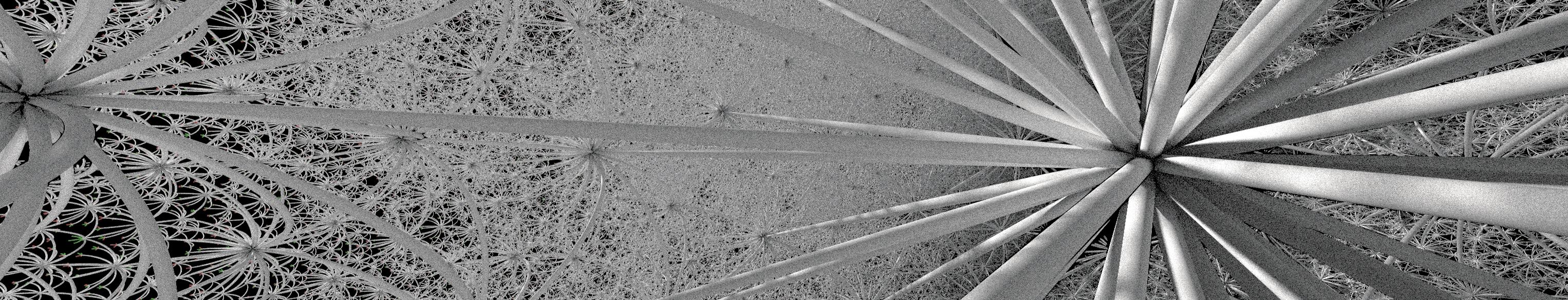
All of the full width images were created using Fragmentarium, which comes with several of Knighty's scripts. The source for this page can be found on Github.
Links
Jenn 3D (2001-2007) by Fritz Obermeyer.
Knighty's fold method (Fractal Forums thread from 2012).
Abdelaziz Nait Merzouk (Knighty) on Google Plus
My introduction to distance estimation.
Jos Leys has also written about the
construction of 4D polytopes - the page looks great, but is in French!
Cayley graphs short introduction to Cayley graphs.
Todd Coxeter algorithm using the Schreier graph approach (which is used by Jenn 3D).
Meaning of regular polytope explains what
flags and transitive symmetries are.
What is the Coxeter diagram for? (StackExchange)
An introduction to computational group theory
Generating and Rendering Four-Dimensional Polytopes
John M. Sullivan (1990).
Roice Nelson has some great visualizations (several being used on Wikipedia).
Wikipedia has lots of (good) information: Uniform polytope, Todd-Coxeter algorithm, Coxeter group, Coxeter-Dynkin diagram, Polyhedron, Honeycombs
I have also heard good things about John Conway's The symmetries of things, but I haven't read it myself.